
Looking at 2019 NFC East Offensive Spending vs. Production with nflfastR
I have been following nflscrapR and NFL analytics community on Twitter for a while now and digging into the package has long been an item on my to-do list. With a lot more free time on my hands due to the pandemic and the recent release of nflfastR, a new package which builds on nflscrapr, I decided it was time to dive in.
If you are not familiar nflscrapR, and now nflfastR, are packages that pull play-by-play data from the NFL API and then parse the text description of each play to give you a cleaned up, analysis ready dataset. Open source sports data is hard to come by so the package(s) and community around them have become quite popular. On top of the play-by-play data they also includes built in models such as Expected Points (EP) and Win Probability (WP).
If you are not familiar with EP or WP the original paper is available here. To summarize:
Expected Points
At its core EP looks at the current in-game situation and, using a model trained on historical play-by-play data, says based on the current in-game situation what do teams typically go on to do. To accomplish this EP uses a multinomial logistic regression model to estimate the expected points for a given situation. It takes the following input features:
-Current down
-Number of seconds remaining in the half
-Yards from the endzone
-A log transform of yards to go for a first down
-A binary indicator for whether or not it is a goal down situation
-Another binary indicator for whether or not there is less than two minutes remaining in the half
The model uses these features, which describe the current in-game drive situation, to estimate the probabilities of the response variable which in this scenario is every possible drive outcome:
-Touchdown (7)
-Field Goal (3)
-Safety (2)
-No Score (0)
- (−) Touchdown (-7)
- (−) Field Goal (-3)
- (−) Safety (-2)
Finally it takes these predicted probabilities and multiplies them by their respective point values to get the Expected Points of that particular situation.
Win Probability
WP follows the same framework but instead of asking what do teams go on to do during a drive in this situation it asks how often does a team in this situation win the game. WP also uses a different model, a generalized additive model, as well as a different set of features to describe the game state:
-Expected score differential
-Number of seconds remaining in game
-Expected score time ratio
-Current half of the game (1st, 2nd, or overtime)
-Number of seconds remaining in half
-Indicator for whether or not time remaining in half is
under two minutes
-Time outs remaining for offensive (possession) team
-Time outs remaining for defensive team
EPA and WPA
With both EP and WP the core value comes when you look at the difference in values between two plays. If you consider the current play Vi and the following play Vf you can place either EP or WP in and calculate Vf-Vi to determine the Expected Points Added (EPA) and WPA (Win Probability Added) of that particular play. As an Eagles fan I particularly enjoyed this example from the paper:
During Super Bowl LII the Philadelphia Eagles’ Nick Foles received a touchdown when facing fourth down on their opponent’s one yard line with thirty-eight seconds remaining in the half. At the start of the play the Eagles’ expected points was V i ≈ 2.78, thus resulting in EPA ≈ 7 − 2.78 = 4.22. In an analogous calculation, this famous play known as the “Philly special” resulted in WPA ≈ 0.1266 as the Eagles’ increased their lead before the end of the half.
2019 NFC East Offensive Spending
For my own analysis I wanted to look into the 2019 NFC East offensive spending and see how offensive production compared. I was able to pull salary data from spotrac to put together the below chart on spending by team and position.
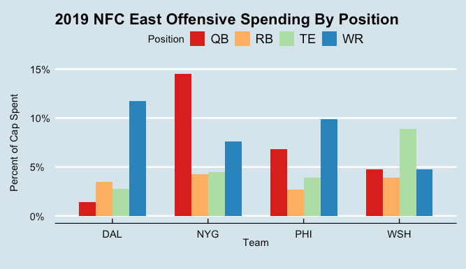
Some quick takeaways from this:
-Dak was on the last year of his rookie contract so the Cowboys were spending very little on quarterbacks.
-On the other end of the spectrum Eli Manning was also on the final year of his deal but took home 23M or almost 12% of the entire Giants cap space.
-All four teams in the division spent roughly the same amount on running backs.
-Washington spent nearly double the rest of division on tight ends with Jordan Reed and Vernon Davis both on lucrative deals, both of whom ended up on the IR.
-Dallas spent the most out of the group in wide receivers - and for good reason.
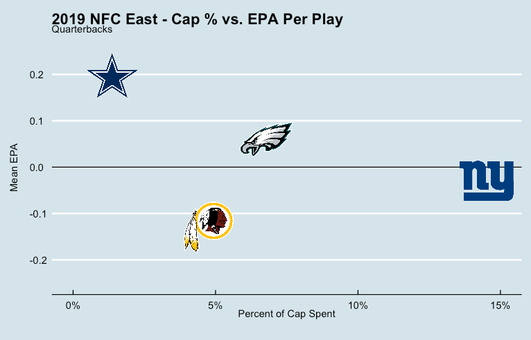
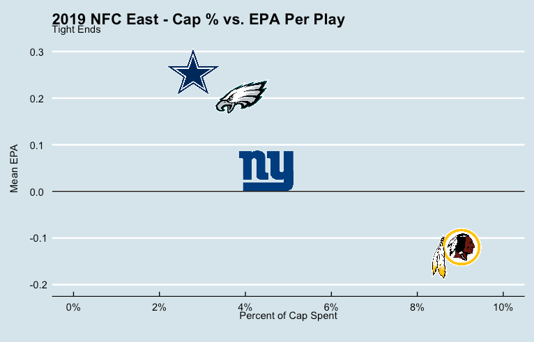
Spending vs. Production
Next I wanted to see how this spending compared to the offensive output of each position. To do this I looked at the average EPA per play by position and compared it to the cap % spent. I should state that this approach is rather crude and does have its limitations:
- EPA is based on the outcome of the entire play which consists of 11 offensive players. Theoretically the credit should be divided among these players and not given solely to the one key offensive player involved.
- You need to consider certain players contracts in the context of their career progression like Dak and Eli.
That being said EPA can work well as a proxy measure and I thought this would be an interesting way to get my feet wet with NFL data.
Takeaways:
Quarterbacks - Its hard to gauge too much here due to Dak and Eli's situations but you can see just how valuable Dak was to the Cowboys and that they're going to have to empty the bank to secure him long term.
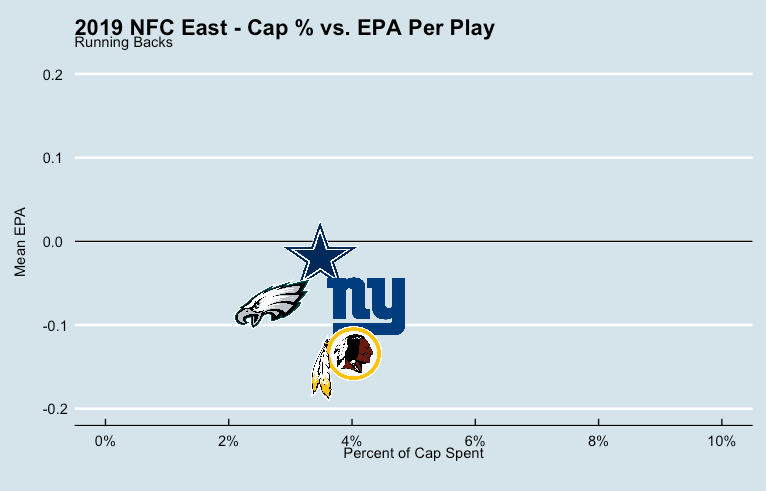
Running Backs - All four teams are pretty tightly clustered here which is in line with the NFL analytics communities darling mantra that running backs don't matter.
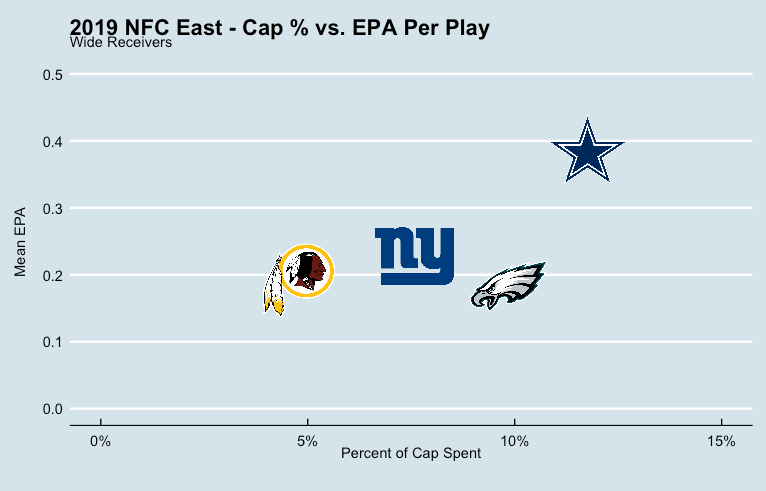
Wide Receivers - Washington, New York and Philadelphia paid between five to ten percent of cap on their receivers and all got roughly the same output while the Cowboys paid a bit more and got significantly higher output from their star receiving core.
Tight Ends - Washington spent more than twice the rest of the division on tight ends and ended up with an average EPA per play less the -.1. This was mostly due to bad fortune with Jordan Reed and Vernon Davis both suffering concussions and missing all or most of the season respectively.
While this analysis was interesting I think a logical next step with would be to factor in offensive line ratings for each team as you can imagine a good line will: give the quarterback more time in the pocket, create more room for running backs, and give tight ends and receivers more time to run their routes. This would alleviate some of the credit distribution issues without getting into more complex modeling. It would also be interesting to look more into individual players and their value as well as how this changes throughout their career.
If you have any questions, feedback, advice, or corrections please get in touch with me on Twitter or email me - link on sidebar. Also wanted to give a shoutout to the developers of both nflscrapR and nflfastR for creating such useful tools that allow anyone to get involved in the NFL data world.